Plot Bland-Altman statistics
Arguments
- data
A data frame
- var1
1st variable to compare (unquoted)
- var2
2nd variable to compare (unquoted)
- label
data label (unquote)
- group
grouping variable used for faceting (unquoted)
- colour
colour asthetic for scatter points (unquoted)
- shape
shape asthetic for scatter points (unquoted)
- xlab
The text for the x-axis label
- ylab
The text for the y-axis label
- title
plot title
- caption
plot caption
- alpha
alpha level for the intervals
Value
ggplot2::ggplot object
See also
Examples
library(tidyr)
tbl <- temperature %>% pivot_wider(names_from = method, values_from = temperature)
# simple example
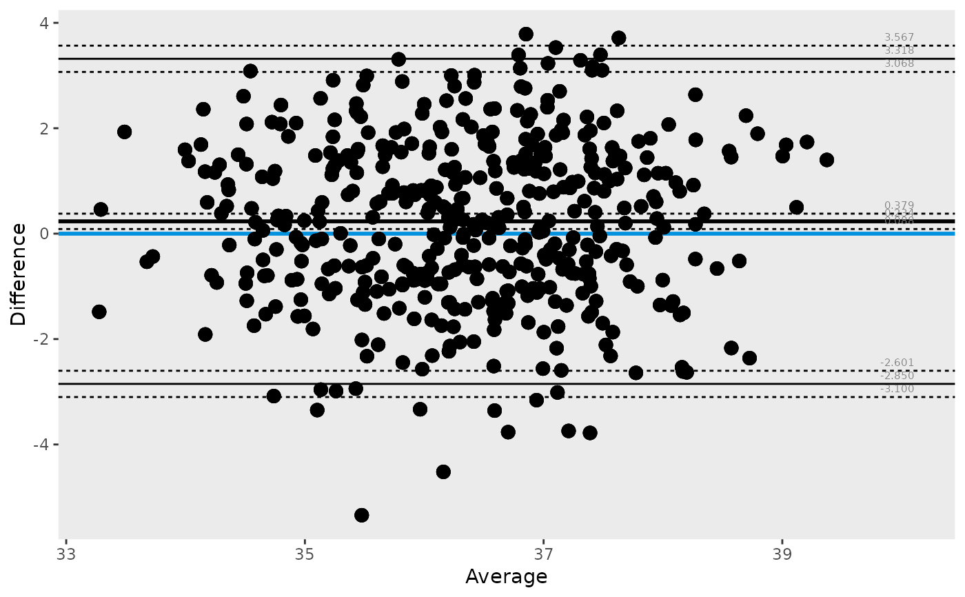
ba_plot(data = tbl, var1 = infrared, var2 = rectal)
 # with colors
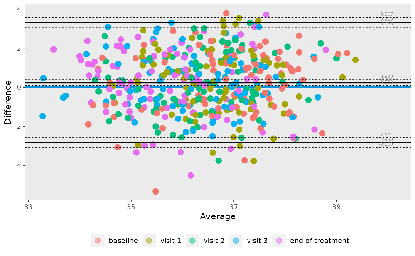
ba_plot(data = tbl, var1 = infrared, var2 = rectal, colour = visit)
# with colors
ba_plot(data = tbl, var1 = infrared, var2 = rectal, colour = visit)
 # with colors and faceting
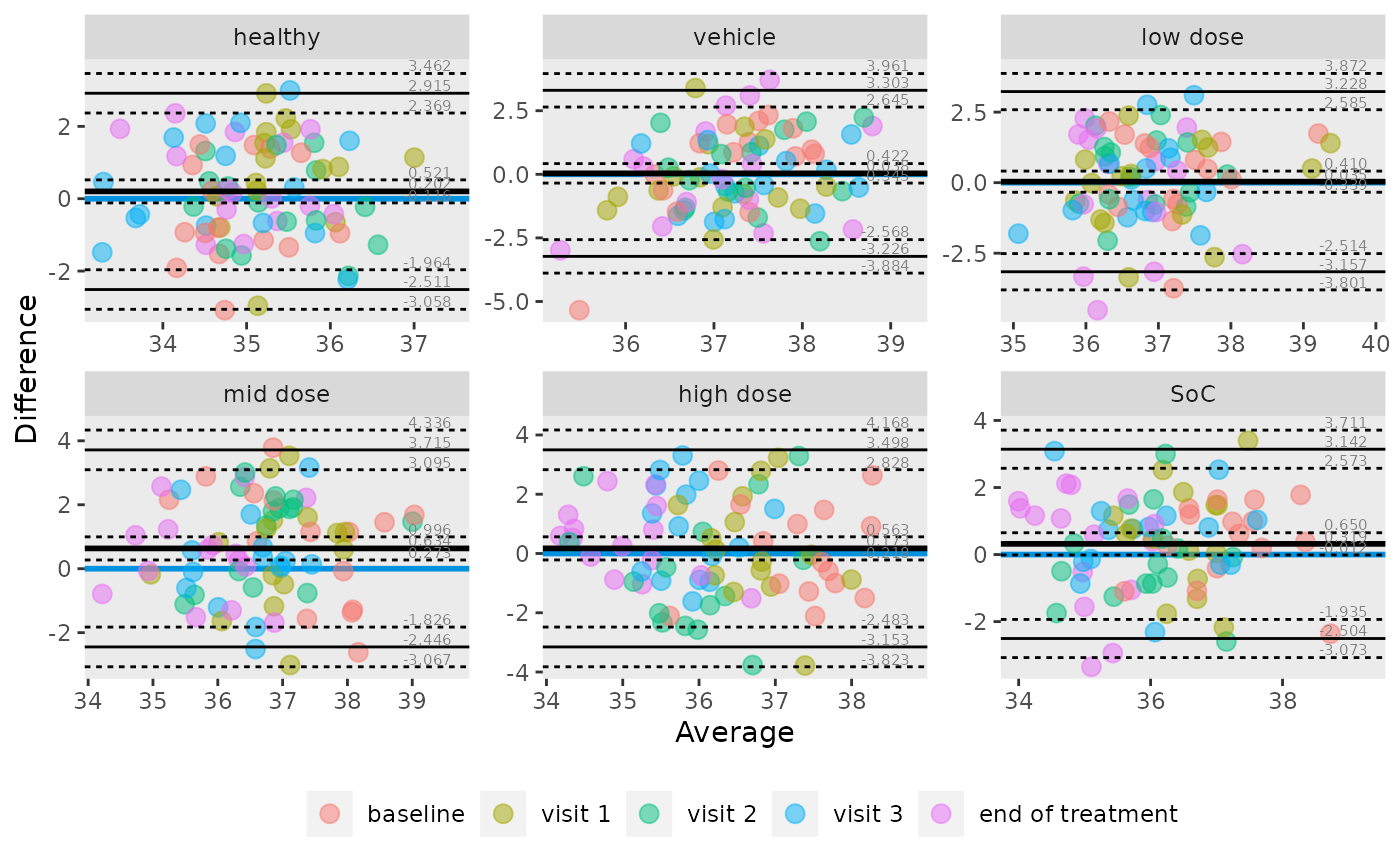
ba_plot(data = tbl, var1 = infrared, var2 = rectal, group = treatment, colour = visit)
# with colors and faceting
ba_plot(data = tbl, var1 = infrared, var2 = rectal, group = treatment, colour = visit)