Compare methods across analysis scales

Overview

library(dplyr)
#> 
#> Attaching package: 'dplyr'
#> The following objects are masked from 'package:stats':
#> 
#>     filter, lag
#> The following objects are masked from 'package:base':
#> 
#>     intersect, setdiff, setequal, union
library(knitr)
library(tidyr)
library(ggBA)

This vignette compares the same two measurement methods under three transformations:

1. identity: absolute differences on the original scale
2. log: ratio-focused agreement
3. logit: agreement for proportion-scale measurements

Prepare paired data

tbl <- temperature |>
  pivot_wider(names_from = method, values_from = temperature)

The temperature dataset is stored in long format (method + temperature values). For pairwise comparisons, we first create one column per method (infrared, rectal).

Identity scale (default)

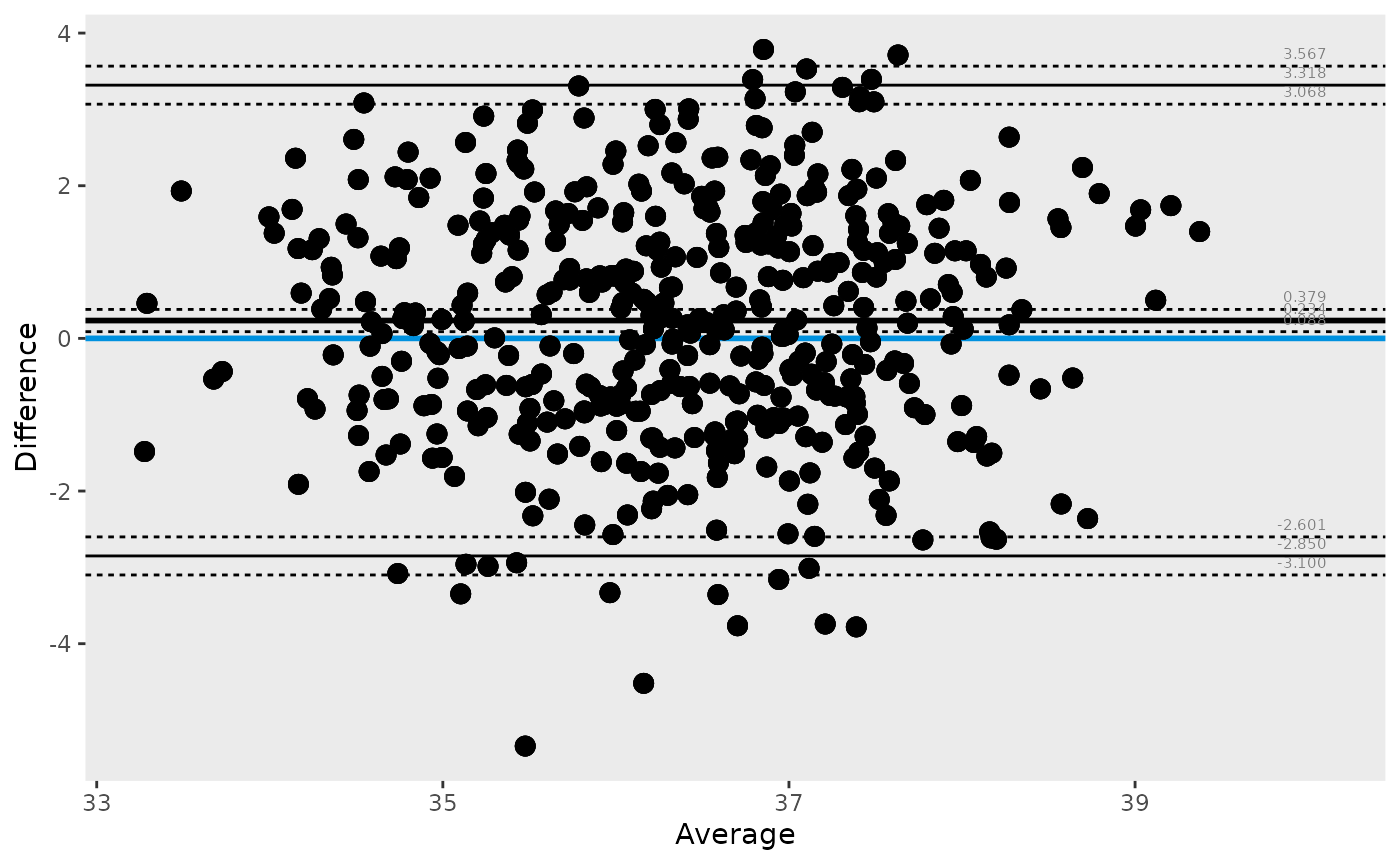
Use this when absolute differences are directly interpretable.

ba_stat(data = tbl, var1 = infrared, var2 = rectal) |>
  pivot_wider(names_from = parameter, values_from = value) |>
  kable(digits = 3)

n	bias	lloa	uloa	bias.lcl	lloa.lcl	uloa.lcl	bias.ucl	lloa.ucl	uloa.ucl
450	0.234	-2.85	3.318	0.088	-3.1	3.068	0.379	-2.601	3.567

ba_plot(data = tbl, var1 = infrared, var2 = rectal)
#> Warning: Using `by = character()` to perform a cross join was deprecated in dplyr 1.1.0.
#> ℹ Please use `cross_join()` instead.
#> ℹ The deprecated feature was likely used in the ggBA package.
#>   Please report the issue to the authors.
#> This warning is displayed once per session.
#> Call `lifecycle::last_lifecycle_warnings()` to see where this warning was
#> generated.

Log scale

Use a log transform when proportional differences are more meaningful than absolute ones. On this scale:

log(var1) - log(var2) = log(var1 / var2)

log_stats <- ba_stat(data = tbl, var1 = infrared, var2 = rectal, transform = "log")

log_stats |>
  pivot_wider(names_from = parameter, values_from = value) |>
  kable(digits = 4)

n	bias	lloa	uloa	bias.lcl	lloa.lcl	uloa.lcl	bias.ucl	lloa.ucl	uloa.ucl
450	0.0064	-0.0784	0.0912	0.0024	-0.0853	0.0843	0.0104	-0.0715	0.0981

The bias can be back-transformed to a ratio: exp(bias) gives the geometric mean ratio (infrared / rectal).

log_bias <- log_stats |>
  filter(parameter == "bias") |>
  pull(value)
cat("Geometric mean ratio (infrared / rectal):", round(exp(log_bias), 4), "\n")
#> Geometric mean ratio (infrared / rectal): 1.0064

ba_plot(
  data      = tbl,
  var1      = infrared,
  var2      = rectal,
  transform = "log",
  xlab      = "Mean of log(temperature)",
  ylab      = "log(infrared / rectal)"
)

Logit scale for proportions

For values restricted to (0, 1), a logit transform often gives better variance behavior and an approximately Normal difference scale.

set.seed(42)
prop_tbl <- data.frame(
  p1 = runif(60, 0.05, 0.95),
  p2 = runif(60, 0.05, 0.95)
)

logit_stats <- ba_stat(data = prop_tbl, var1 = p1, var2 = p2, transform = "logit")

logit_stats |>
  pivot_wider(names_from = parameter, values_from = value) |>
  kable(digits = 3)

n	bias	lloa	uloa	bias.lcl	lloa.lcl	uloa.lcl	bias.ucl	lloa.ucl	uloa.ucl
60	0.441	-3.546	4.427	-0.085	-4.449	3.524	0.966	-2.643	5.33

ba_plot(
  data      = prop_tbl,
  var1      = p1,
  var2      = p2,
  transform = "logit",
  xlab      = "Mean of logit(proportion)",
  ylab      = "Difference on logit scale"
)